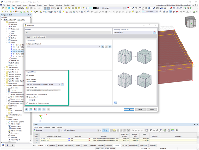
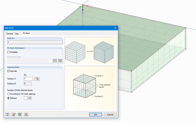
For the meshing of solids, you have the option of arranging a layered FE mesh. This option allows you to perform a defined division of the solid with finite elements between two parallel surfaces.
Go to Explanatory Video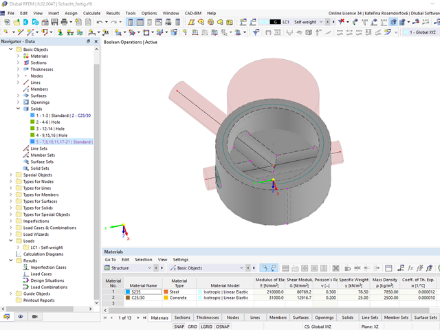
Curved elements are available only in RFEM. It's possible to intersect curved surfaces and solids.
When doing this, the program generates surfaces with the "Trimmed" surface type. With this technology, you can create very complex geometries, such as pipe intersections or curved openings, with a single click.
The intersection of solids is carried out adaptively using the new solid types "Hole" and "Intersection", according to the set theory. Use this method to create new, complex solid geometries similar to the manufacturing process (drilling, milling, turning, etc.). Therefore, it is possible to create complex curved surface or perforated solid elements. It's a simple process!
Go to Explanatory Video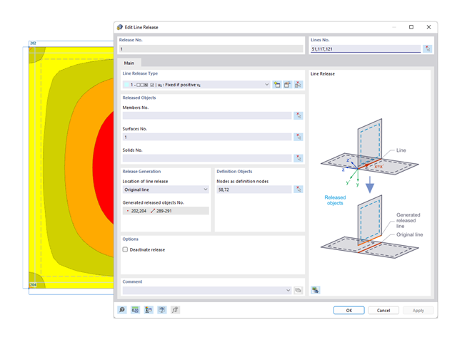
You probably already know that node, line, and surface releases are used to define transfer conditions between objects. For example, you can release members, surfaces, and solids from a line. It is also easily possible for the releases to have nonlinear properties, such as "Fixed if positive n", "Fixed if negative n", and so on.
.png?mw=640&hash=55038d2a1591f62179796666cb9b2fede0274e19)
A graphical and tabular output of the results for deformations, stresses, and strains helps you when determining the soil solids. To achieve this, use the special filter criteria for targeted selection of results.
The program doesn't leave you alone with the results. If you want to graphically evaluate the results in the soil solids, you can use the guide objects. For example, you can define clipping planes. This allows you to view the corresponding results in any plane of the soil solid.
And not just that. The utilization of result sections and clipping boxes facilitates the precise graphical analysis of the soil solid.

The soil solids that you want to analyze are summarized in soil massifs.
Use the soil samples as a basis for a definition of the respective soil massif. This way, the program allows for user-friendly generation of the massif, including the automatic determination of the layer interfaces from the sample data, as well as the groundwater level and the boundary surface supports.
Soil massifs provide you with the option to specify a target FE mesh size independently of the global setting for the rest of the structure. You can thus consider the various requirements of the building and soil in the entire model.
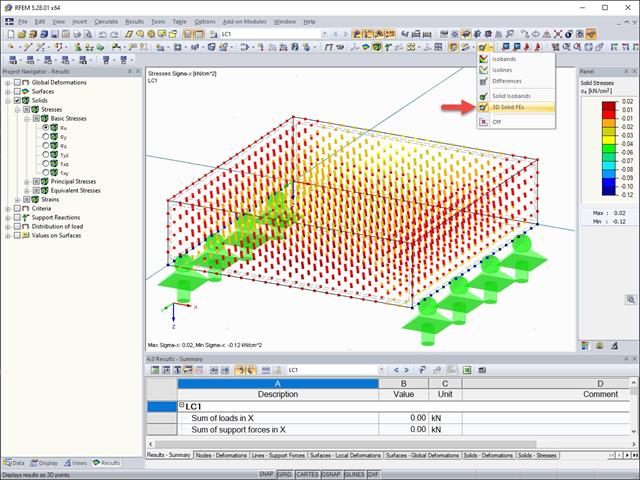
The results of solid stresses can be displayed as colored 3D points in the finite elements.
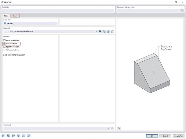
In addition to the "Mesh Refinement" and "Specific Direction" options for solids, you can also activate the "Grid for Results" option, which allows for organizing grid points in the solid space. Among other things, the center of gravity can be set as the origin. There is also the option to activate or deactivate the visibility of the grid for numerical results in "Navigator – Display" under Basic Objects.
.png?mw=640&hash=342149908caead326e60e26a2b5d05f7f46825cb)
Are you familiar with the Tsai-Wu material model? It combines plastic and orthotropic properties, which allows for special modeling of materials with anisotropic characteristics, such as fiber-reinforced plastics or timber.
If the material is plastified, the stresses remain constant. The redistribution is carried out according to the stiffnesses available in the individual directions. The elastic area corresponds to the Orthotropic | Linear Elastic (Solids) material model. For the plastic area, the yielding according to Tsai-Wu applies:
All strengths are defined positively. You can imagine the stress criterion as an elliptical surface within a six-dimensional space of stresses. If one of the three stress components is applied as a constant value, the surface can be projected onto a three-dimensional stress space.
If the value for fy(σ), according to the Tsai-Wu equation, plane stress condition, is smaller than 1, the stresses are in the elastic zone. The plastic area is reached as soon as fy (σ) = 1; values greater than 1 are not allowed. The model behavior is ideal-plastic, which means there is no stiffening.

Did you know? In contrast to other material models, the stress-strain diagram for this material model is not antimetric to the origin. You can use this material model to simulate the behavior of steel fiber-reinforced concrete, for example. Find detailed information about modeling steel fiber-reinforced concrete in the technical article about Determining the material properties of steel-fiber-reinforced concrete.
In this material model, the isotropic stiffness is reduced with a scalar damage parameter. This damage parameter is determined from the stress curve defined in the Diagram. The direction of the principal stresses is not taken into account. Rather, the damage occurs in the direction of the equivalent strain, which also covers the third direction perpendicular to the plane. The tension and compression area of the stress tensor is treated separately. In this case, different damage parameters apply.
The "Reference element size" controls how the strain in the crack area is scaled to the length of the element. With the default value zero, no scaling is performed. Thus, the material behavior of the steel fiber concrete is modeled realistically.
Find more information about the theoretical background of the "Isotropic Damage" material model in the technical article describing the Nonlinear Material Model Damage.
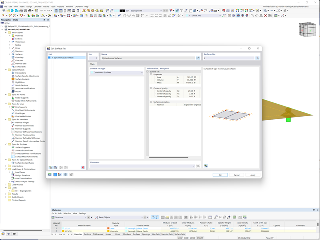
The aim of this feature is to make your design more efficient. In addition to member sets, you can also combine lines, surfaces, and solids into sets. For example, you can consider them as uniform elements in the design.
RFEM is entering a new phase with RFEM 6! The new generation of the 3D FEA software is also used for the structural analysis of members, surfaces, and solids. Many of the tried and tested features remain, but we have improved them and added new features to make your work with RFEM even easier.
What particularly distinguishes RFEM 6 is the modern design concept, with the add-ons integrated directly into the program. Curious to learn more?
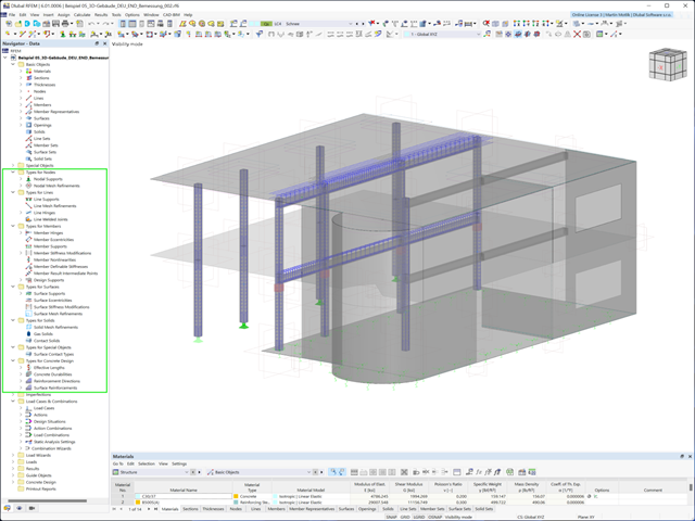
Use the specification of the element types for members, surfaces, solids, and so on, to facilitate your input (such as member nonlinearities, member stiffnesses, design supports, and many others).

Compared to the RF‑/STEEL add-on module (RFEM 5 / RSTAB 8), the following new features have been added to the Stress-Strain Analysis add-on for RFEM 6 / RSTAB 9:
- Treatment of members, surfaces, solids, welds (line welded joints between two and three surfaces with subsequent stress design)
- Output of stresses, stress ratios, stress ranges, and strains
- Limit stress depending on the assigned material or a user-defined input
- Individual specification of the results to be calculated through freely assignable setting types
- Non-modal result details with prepared formula display and additional result display on the cross-section level of members
- Output of the design check formulas used

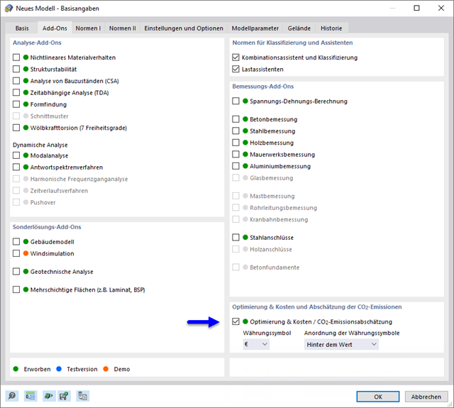
Did you know that The structural optimization in the programs RFEM and RSTAB is a completion of the parametric input. It is a parallel process beside the actual model calculation with all its regular calculation and design definitions. The add-on assumes that your model or block is built with a parametric context and is controlled in its entirety by global control parameters of the "optimization" type. Therefore, these control parameters have a lower and upper limit and a step size to delimit the optimization range. If you want to find optimal values for the control parameters, you have to specify an optimization criterion (for example, minimum weight) with the selection of an optimization method (for example, particle swarm optimization).
You can already find the cost and CO2 emission estimation in the material definitions. You can activate both options individually in each material definition. The estimation is based on a unit for unit cost or unit emission for members, surfaces, and solids. In this case, you can select whether to specify the units by weight, volume, or area.
Both optimization methods have one thing in common. At the end of the process, they provide you with a list of model mutations from the stored data. Here you can find the details of the controlling optimization result and the associated value assignment of the optimization parameters. This list is organized in descending order. You can find the assumed best solution shown in the first line. For this, the optimization result with its determined value assignment is closest to the optimization criterion. All add-on results have a utilization < 1. Furthermore, once the analysis is completed, the program will adjust the value assignment to that of the optimal solution for the optimization parameters in the global parameter list.
In the material dialog boxes, you can find the additional tabs "Cost Estimation" and "Estimation of CO2 Emissions". They show you the individual estimated sums of the assigned members, surfaces, and solids per unit weight, volume, and area. Furthermore, these tabs show the total cost and emission of all assigned materials. This gives you a good overview of your project.

- Automatic consideration of masses from self-weight
- Direct import of masses from load cases or load combinations
- Optional definition of additional masses (nodal, linear, or surface masses, as well as inertia masses) directly in the load cases
- Optional neglect of masses (for example, mass of foundations)
- Combination of masses in different load cases and load combinations
- Preset combination coefficients for various standards (EC 8, SIA 261, ASCE 7,...)
- Optional import of initial states (for example, to consider prestress and imperfection)
- Structure Modification
- Consideration of failed supports or members/surfaces/solids
- Definition of several modal analyses (for example, to analyze different masses or stiffness modifications)
- Selection of mass matrix type (diagonal matrix, consistent matrix, unit matrix), including user-defined specification of translational and rotational degrees of freedom
- Methods for determining the number of mode shapes (user-defined, automatic - to reach effective modal mass factors, automatic - to reach the maximum natural frequency - only available in RSTAB)
- Determination of mode shapes and masses in nodes or FE mesh points
- Results of eigenvalue, angular frequency, natural frequency, and period
- Output of modal masses, effective modal masses, modal mass factors, and participation factors
- Masses in mesh points displayed in tables and graphics
- Visualization and animation of mode shapes
- Various scaling options for mode shapes
- Documentation of numerical and graphical results in printout report

Entering soil layers for soil samples is performed in a clearly arranged dialog box. A corresponding graphical representation supports clarity and makes checking the input user-friendly.
An extensible database facilitates the selection of soil material properties. The Mohr-Coulomb model as well as a nonlinear model with stress and strain dependent stiffness are available for a realistic modeling of the soil material behavior.
You can define any number of soil samples and layers. The soil is generated from all entered samples using 3D solids. Assignment to the structure is carried out using coordinates.
The soil body is calculated according to the nonlinear iterative method. The calculated stresses and settlements are displayed graphically and in tables.
Did you know? When unloading the structural component with a plastic material model, in contrast to the Isotropic | Nonlinear Elastic material model, the strain remains after it has been completely unloaded.
You can select three different definition types:
- Standard (definition of the equivalent stress under which the material plastifies)
- Bilinear (definition of the equivalent stress and strain hardening modulus)
- Stress-strain diagram: definition of polygonal stress-strain diagram
- Option to save / import the diagram
- Interface with MS Excel
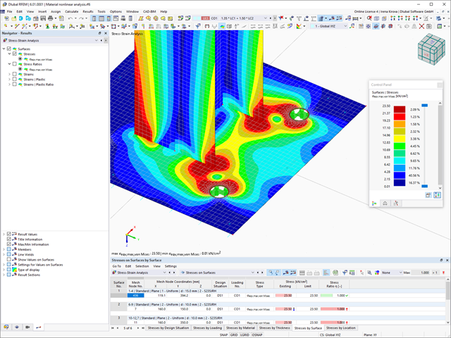
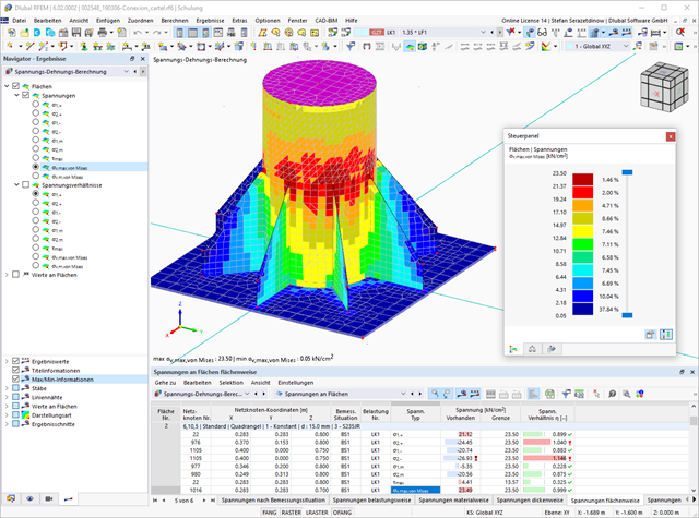
- Determination of principal and basic stresses, membrane and shear stresses, as well as equivalent stresses and equivalent membrane stresses
- Stress analysis for structural surfaces including simple or complex shapes
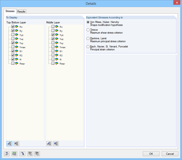
- Equivalent stresses calculated according to different approaches:
- Shape modification hypothesis (von Mises)
- Shear stress hypothesis (Tresca)
- Normal stress hypothesis (Rankine)
- Principal strain hypothesis (Bach)
- Optional optimization of surface thicknesses and data transfer to RFEM
- Output of strains
- Detailed results of individual stress components and ratios in tables and graphics
- Filter function for solids, surfaces, lines, and nodes in tables
- Transversal shear stresses according to Mindlin, Kirchhoff, or user-defined specifications
- Stress evaluation for welds at connection lines between surfaces (see the Product Feature)
If you release a structural component with a nonlinear elastic material again, the strain goes back on the same path. In contrast to the Isotropic|Plastic material model, there is no strain left when completely unloaded.
You can select three different definition types:
- Standard (definition of the equivalent stress under which the material plastifies)
- Bilinear (definition of the equivalent stress and strain hardening modulus)
- Stress-Strain Diagram:
- Definition of polygonal stress-strain diagram
- Option to save / import the diagram
- Interface with MS Excel
Background information about nonlinear material models can be found in the technical article describing the yield laws in isotropic nonlinear elastic material model.
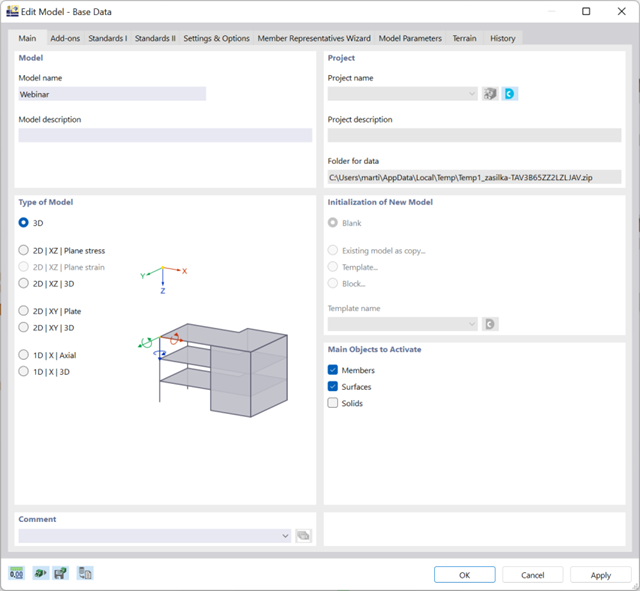
There are many options available for simple input and modeling. Your model is entered as a 1D, 2D, or 3D model. Member types such as beams, trusses, or tension members make it easier for you to define member properties. In order to model surfaces, RFEM provides you with various types, such as Standard, Without Thickness, Rigid, Membrane, and Load Distribution.
Furthermore, RFEM covers various material models, such as Isotropic | Linear Elastic, Orthotropic | Linear Elastic (Surfaces, Solids), or Isotropic | Timber | Linear Elastic (Members).
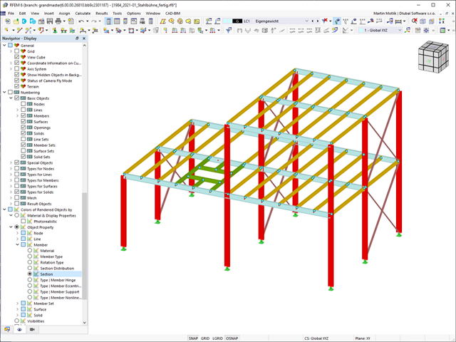
It is possible to assign different colors to various objects of a structure in order to make the rendering display of the structure more clearly arranged.
A distinction is made between the various object properties of nodes, lines, members, member sets, surfaces, and solids. Moreover, the model can be displayed in photorealistic rendering.
Go to Explanatory Video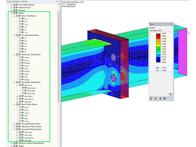
Display extended strains of members, surfaces, and solids (for example, the important principal strains, equivalent total strains, and so on) in the Project Navigator - Results in RFEM as well as in Table 4.0.
For example, you can display governing plastic strains when performing the plastic design of connections with surface elements.
The stiffness of gas given by the ideal gas law pV = nRT can be considered in the nonlinear dynamic analysis.
The calculation of gas is available for accelerograms and time diagrams for both the explicit analysis and the nonlinear implicit Newmark analysis. To determine the gas behavior correctly, at least two FE layers for gas solids should be defined.
The global calculation assigns the stiffness determined by means of the selected composition and the glass geometry to each surface. Then, the calculation proceeds using the plate theory. It is possible to select whether the shear coupling of layers should be considered.
In the case of the local calculation, you can further specify 2D or 3D calculation. Two-dimensional calculation means that the single-layer or laminated glass is modeled as a surface, whose thickness is calculated on the basis of the selected structure and glass geometry (using the plate theory). Similarly to the global calculation, you can optionally consider shear coupling of layers.
The 3D calculation uses solids in the model to substitute each composition layer. This way, the results are more accurate, but the calculation may take more time.
It is possible to model insulating glass only if local calculation is selected. The gas layer is always modeled as a solid element, so it is necessary to design individual insulating glass parts independently of the surrounding structure. The ideal gas law (thermal equation of state of ideal gases) is considered for the calculation and the third-order analysis.
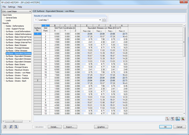
After the calculation, you can evaluate the results of the individual load steps directly in the module windows or graphically in a structural model.
The results include, for example, deformations, stresses, and internal forces of surfaces, as well as deformations and stresses of solids. It is possible to export the result combinations for each load step to RFEM. You can use these enveloping combinations for further designs in the other RFEM add-on modules.
All input data and results of the add-on module are part of the global RFEM printout report.